Start with the Basics - Thermodynamics
Everything that happens in the physical world requires energy, from chemical reactions to mechanical processes to biological functions. That energy is never fully recovered and thus moves in one direction, from concentrated usable forms to dispersed, degraded heat.
You don't get energy for free.
(1st Law of Thermodynamics)
Energy is conserved. It cannot be created from nothing. It can only change form. There is no perpetual motion machine, no infinite source, and no technology that generates more energy than it receives. Every promise of unlimited growth through clever innovation is at its core a claim that this law does not apply, and all evidence suggests it does.
You lose usable energy every time you use it.
(2nd Law of Thermodynamics)
Every time energy converts from one form to another, such as burning fuel, running a motor, digesting food, or firing a neuron, some of it disperses as waste heat. That dispersal is permanent, meaning it cannot be reversed. The universe's stock of ordered, usable energy is always, irreversibly declining.
You can never eliminate losses completely.
(3rd Law of Thermodynamics)
Efficiency can improve. Engines get better, insulation gets thicker, transmission losses shrink. But 100% efficiency is not an engineering challenge. It is a physical impossibility. There is always a cost to using energy, and that cost can never be zero.
Law one destroys the idea of infinite growth. Law two is the arrow of time: every process costs more than the work it does, and there is no going back. Law three indicates that improvement can occur but losses are inevitable. These are not the opinions of scientists with a particular worldview. They are the most rigorously tested framework in the history of physics.
Every complex process requires a fresh energy gradient, ie a source of concentrated energy. The quality, as well as quantity, of that energy source determines how much useful work can be done.

A Practical Introduction to Entropy
Dissipative Structures
Given the constraints of thermodynamics, how does complexity exist at all?
The answer is that organized systems are not stable objects, but ongoing processes that maintain their form by continuously consuming energy and expelling waste. Ilya Prigogine called these dissipative structures and his work on this earned him the 1977 Nobel Prize in Chemistry. Recognizable examples includes hurricanes, living cells, ecosystems, and human civilization.
One of the essential characteristics of dissipative structures is that they exist far from equilibrium, thermodynamically. They actively resists the universe’s tendency toward disorder. They are open systems that require constant energy input and waste output. Order is maintained by accelerating entropy production elsewhere. Dissipative structures involve irreversible processes in their formation such that energy flows “downhill” while maintaining organized complexity. Structure are spontaneously self-organize. In other words, the internal dynamics generate the pattern (or emergent state) when conditions are met.
The key insight is that all complex organization exists by accelerating the dispersal of energy gradients. The organization is not stored anywhere, it is being actively re-purchased, every moment, by throughput.
A hurricane persists when it efficiently dissipates the temperature difference between tropical ocean and upper atmosphere. A cell maintains its organization by burning glucose and producing heat and waste. A city sustains its infrastructure by consuming energy and generating waste.
Dissipative structures require continuous energy throughput to persist. There’s no “steady state” at reduced energy flow. You cannot build a structure on high energy availability and then maintain it on low energy availability.The structure’s complexity scales with energy throughput. The maintenance requirement scales with structure complexity.
A candle flame has a consistent, recognizable shape, but that shape is a process. Interrupt the fuel supply, and the structure doesn’t just weaken, it ceases. The apparent stability of these systems is dynamic. There is no resting state without continuous energy throughput.
Dissipative structures exhibit non-linear dynamics. Small perturbations can product large effects, and outputs are not proportional to inputs. This creates emergent conditions at critical thresholds, easily recognizable in systems like hurricanes, fire, tornadoes, etc.
Industrial civilization is a dissipative structure sustained by ~600 exajoules annually, ~80% from fossil fuels (Energy Institute, 2024).This structure includes 8 billion humans, global supply chains, electricity grids, water systems, and vast infrastructure networks. When energy throughput to a dissipative structure decreases, the typical trajectory is not gradual decline but relatively rapid simplification to a lower organizational state that matches available energy flow. This is a pattern observed in ecosystem regime shifts (Scheffer et al., 2001), the adaptive cycles of social-ecological systems (Holling, 2001), and historical civilizational collapses (Tainter, 1988; Homer-Dixon, 2006).
Understanding civilization as a dissipative structure clarifies what adaptation actually means: building different structures suited to available energy flows, not attempting to maintain current complexity indefinitely. Complexity is thermodynamically expensive and cannot be maintained without the energy subsidy that produced it (Prigogine & Stengers, 1984; Odum, 1996). This principle is foundational to biophysical economics (Georgescu-Roegen, 1971; Hall et al., 1986), metabolic ecology (Brown et al., 2004), and energy history (Smil, 2017).

-
Prigogine, Ilya & Stengers, Isabelle. Order Out of Chaos: Man's New Dialogue with Nature. 1984. Bantam Books.
Tainter, Joseph A. The Collapse of Complex Societies. Cambridge University Press, 1988.
Holling, C.S. “Understanding the Complexity of Economic, Ecological, and Social Systems.” Ecosystems 4, no. 5 (2001): 390-405.
Scheffer, Marten, et al. “Catastrophic Shifts in Ecosystems.” Nature 413 (2001): 591-596.
Homer-Dixon, Thomas. The Upside of Down: Catastrophe, Creativity, and the Renewal of Civilization. Island Press, 2006.
Odum, Howard T. Environmental Accounting: EMERGY and Environmental Decision Making. Wiley, 1996.
Hall, Charles A.S., Cleveland, Cutler J., and Kaufmann, Robert. Energy and Resource Quality: The Ecology of the Economic Process. University Press of Colorado, 1986.
Georgescu-Roegen, Nicholas. The Entropy Law and the Economic Process. Harvard University Press, 1971.
Brown, James H., et al. “Toward a Metabolic Theory of Ecology.” Ecology 85, no. 7 (2004): 1771-1789.
Smil, Vaclav. Energy and Civilization: A History. MIT Press, 2017.
Energy Institute. Statistical Review of World Energy. 2024. https://www.energyinst.org/statistical-review
Understanding Complexity as Dissipative Structures
Energy Return on Investment
Energy return on investment (EROI) is a simple idea dressed in technical language. It asks: how much energy do you have to put in to get energy out?
A farmer understands this intuitively. You plant a bushel of wheat to harvest ten. If conditions deteriorate and you start harvesting five, the farm is in trouble, because the margin has shrunk. Less surplus means less seed for next year, less food for the family, less capacity to withstand a bad season.
So the question is how much energy is left over after the extraction process itself is paid for? Early oil was like a dream harvest. In the 1930s, you invested one barrel’s worth of energy in drilling and refining and got roughly a hundred barrels back. 100:1 (Guilford et al., 2011). That surplus was the engine of the twentieth century. This net energy built the interstate highway system, funded universal public education, expanded hospitals, and created the middle class as a mass phenomenon. The surplus of energy freed up labor from food and shelter production, for education, health, and innovation.
By the 1970s, the ratio had fallen to around thirty to one. By the 1990s, eighteen to one (Guilford et al., 2011). Today, conventional oil runs around eleven to one, and the shale and tight oil that dominate new American production returns somewhere roughly around five to eight to one (Hall et al., 2014). Below this threshold, you begin to lose the surplus energy needed to run the complex civilization built on top of the energy system (Murphy & Hall, 2010; Lambert et al., 2014). The farm starts eating its seed. This is called the “energy cliff.”
Renewable energy like solar and wind estimates vary, with most analyses placing utility-scale solar and wind in the range of 10:1 to 30:1 (Weißbach et al., 2013; Raugei et al., 2017). But the transition from a high-EROI fossil fuel economy to a lower-EROI renewable one requires enormous upfront investment of the very energy and materials that are becoming more costly, restructuring systems built for different energy characteristics, and culturally accepting that the era of near-limitless surplus is not returning regardless of how the transition goes.
This is a net energy cliff effect. As EROI declines, an increasingly large fraction of total energy output must be reinvested in the energy system itself, leaving less for everything else (Hall & Klitgaard, 2012). This is already measurable in the data rather than being a prediction of a future state (King & Hall, 2011).
The margin has shrunk, and that shrinkage is structural. It runs underneath inflation, infrastructure decay, and the emerging sense that the same effort yields less than it used to.
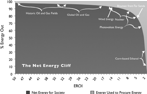
The “ Net Energy Cliff ” with EROI expressed as the number of the horizontal axis to one, i.e. 20:1, adapted from Murphy and Hall (2010)).
-
Guilford, M.C., et al. “A New Long Term Assessment of Energy Return on Investment (EROI) for U.S. Oil and Gas Discovery and Production.” Sustainability 3, no. 10 (2011): 1866-1887.
Hall, Charles A.S. and Klitgaard, Kent A. Energy and the Wealth of Nations: An Introduction to Biophysical Economics. Springer, 2012.
Hall, Charles A.S., Lambert, Jessica G., and Balogh, Stephen B. “EROI of Different Fuels and the Implications for Society.” Energy Policy 64 (2014): 141-152.
King, Carey W. and Hall, Charles A.S. “Relating Financial and Energy Return on Investment.” Sustainability 3, no. 10 (2011): 1810-1832.
Lambert, Jessica G., et al. “Energy, EROI and Quality of Life.” Energy Policy 64 (2014): 153-167.
Murphy, D.J. and Hall, C.A.S. “Year in review—EROI or energy return on (energy) invested.” Annals of the New York Academy of Sciences 1185 (2010): 102–118. https://doi.org/10.1111/j.1749-6632.2009.05282.x
Raugei, Marco, et al. “Energy Return on Energy Invested (ERoEI) for photovoltaic solar systems in regions of moderate insolation: A comprehensive response.” Energy Policy 102 (2017): 377-384.
Weißbach, Daniel, et al. “Energy intensities, EROIs (energy returned on invested), and energy payback times of electricity generating power plants.” Energy 52 (2013): 210-221. here
EROI for visual learners
The Curve - Resource Constrained Growth
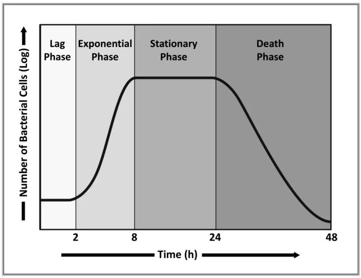
Every system that consumes resources in a bounded space follows the same underlying dynamic. Biologists made it visible in bacterial cultures—exponential growth, overshoot, collapse (Monod, 1949). The same dynamic appears across fisheries (Schaefer, 1954), oil fields (Hubbert, 1956), and civilizations (Catton, 1980; Tainter, 1988), though rarely as cleanly, because real systems intervene, substitute, and delay. The interventions change the shape of the curve.
It has four phases (Monod, 1949). First, a lag where the system establishes itself, grows slowly, explores its environment. Then exponential growth where resources seem effectively unlimited, and the system expands rapidly, doubling and doubling again. Then a stationary phase where growth meets limits, inputs and outputs balance. The system can sustain itself but not expand further. Finally, if the system does not adapt, a death phase where costs exceed inputs, and the system contracts.
We added the first billion people to the planet over all of human history until around 1800. We added the next billion in 130 years. The next in 30 years. We have added more than four billion in the past sixty years (United Nations, 2022). Global energy consumption followed the same shape: essentially flat for millennia, then a hockey stick beginning with the industrial revolution, accelerating through the twentieth century (Smil, 2017; Steffen et al., 2015).
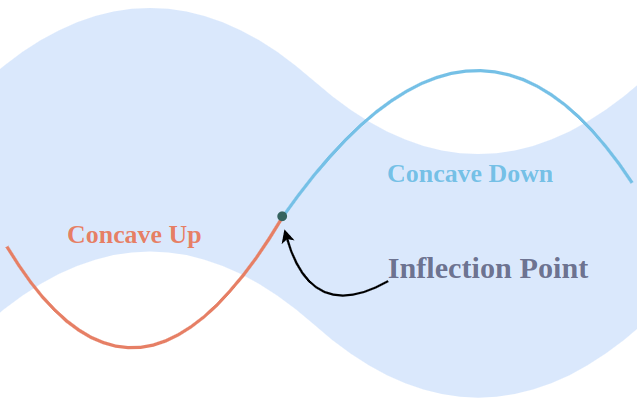
Every exponential growth curve in a finite system has an inflection point, or the place where the curve begins to change direction. Not necessarily a cliff, it’s often a long, gradual bend. But the physics of finite systems guarantees that the curve cannot continue indefinitely (Meadows et al., 1972). There is no exception in the natural record.
There are two possible outcomes from an inflection point: a stationary phase, in which the system reaches a sustainable equilibrium (maintenance of complexity through energy and material throughput); or a death phase, in which it does not (Monod, 1949; Holling, 2001). The difference between these outcomes is not random. It depends on whether the system can negotiate constraint before it is imposed by force (Tainter, 1988; Homer-Dixon, 2006).
This brings us to the fundamental constraint of any environment: carrying capacity (K). When a population grows without limits, it follows a J-shaped exponential growth curve. As resources become scarce or waste accumulates, this expansion is slowed, bending the trajectory into an S-shaped logistic growth curve. The video below is a helpful explanation of these processes.
-
Pearl, Raymond and Reed, Lowell J. “On the Rate of Growth of the Population of the United States since 1790 and Its Mathematical Representation.” Proceedings of the National Academy of Sciences 6, no. 6 (1920): 275-288.
Monod, Jacques. “The Growth of Bacterial Cultures.” Annual Review of Microbiology 3 (1949): 371-394.
Catton, William R., Jr. Overshoot: The Ecological Basis of Revolutionary Change. University of Illinois Press, 1980.
Schaefer, Milner B. “Some Aspects of the Dynamics of Populations Important to the Management of the Commercial Marine Fisheries.” Bulletin of the Inter-American Tropical Tuna Commission 1, no. 2 (1954): 27-56.
Hubbert, M. King. “Nuclear Energy and the Fossil Fuels.” Drilling and Production Practice, American Petroleum Institute (1956): 7-25.
Tainter, Joseph A. The Collapse of Complex Societies. Cambridge University Press, 1988.
Diamond, Jared. Collapse: How Societies Choose to Fail or Succeed. Viking, 2005.
Meadows, Donella H., et al. The Limits to Growth. Universe Books, 1972.
Holling, C.S. “Understanding the Complexity of Economic, Ecological, and Social Systems.” Ecosystems 4, no. 5 (2001): 390-405.
Homer-Dixon, Thomas. The Upside of Down: Catastrophe, Creativity, and the Renewal of Civilization. Island Press, 2006.
Meadows, Donella H., et al. The Limits to Growth. Universe Books, 1972.
Monod, Jacques. “The Growth of Bacterial Cultures.” Annual Review of Microbiology 3 (1949): 371-394.
Smil, Vaclav. Energy and Civilization: A History. MIT Press, 2017.
Steffen, Will, et al. “The Trajectory of the Anthropocene: The Great Acceleration.” The Anthropocene Review 2, no. 1 (2015): 81-98.
Tainter, Joseph A. The Collapse of Complex Societies. Cambridge University Press, 1988.
United Nations, Department of Economic and Social Affairs, Population Division. World Population Prospects 2022: Summary of Results. UN DESA/POP/2022/TR/NO. 3.